Let’s build a Salesforce Deal Predictor (Part 2)
We demonstrate how to go about creating an AI system that can predict the outcomes of Salesforce opportunities using a custom model built with Pytorch from the ground up.
Introduction
This is the second of two articles that demonstrate how to go about creating an AI system that can predict the outcomes of Salesforce opportunities. In part 1 we focussed on data processing and enriching our data to give us a powerful set of features that will give our model the best chance of making accurate predictions.
Now a word of warning - this is quite a technical article and if you’re someone who has some familiarity with Pytorch you’ll be absolutely fine.
Data Processing
Train / Validation / Test splitting
Now we have a dataset that we have enriched to generate additional features, but there are a couple of additional steps that we need to go through before we have a dataset that is ready for training. The first of these is to split the data into a training, validation and test set. In order to do this we have to remember that our dataset contains the histories of all our opportunities and consequently there will be multiple records for each opportunity (representing different points in time in its sales cycle). Therefore we need to split our dataset by opportunity - that is to say we want to avoid having opportunity history records for any given opportunity split across our training, validation and test sets as this would be data leakage and invalidate our validation and test results.
Imputation
Having split the data we can now impute the missing values that we described in part 1. The reason we do this here is to make sure that the validation and test sets are imputed with values calculated from the properties of the training set as this most closely resembles what will happen with live opportunities in production.
Normalisation
We can then move on and normalise our numerical values by subtracting the mean and dividing by the standard deviation. This will ensure that the values for each feature have a mean of zero and unit variance which ultimately will enable the neural network to train more easily.
Tokenisation
Our text based features will be converted into tokens as we’ll be using embeddings to process these in the model itself, which is a far more data efficient and powerful way of treating this data than the sparse vectors that are created with one-hot encoding. Unlike the tokenisers that are commonplace with LLMs ours is just a simple numerical representation of each distinct text value in each column - sometimes this is called label encoding and it’s far simpler than I’ve just made it sound.
Putting it all together
The last thing to do is to convert the data, which if you’re using pandas, will be stored as numpy arrays into Pytorch tensors as everything from here on it going to be in Pytorch land.
Model Architecture

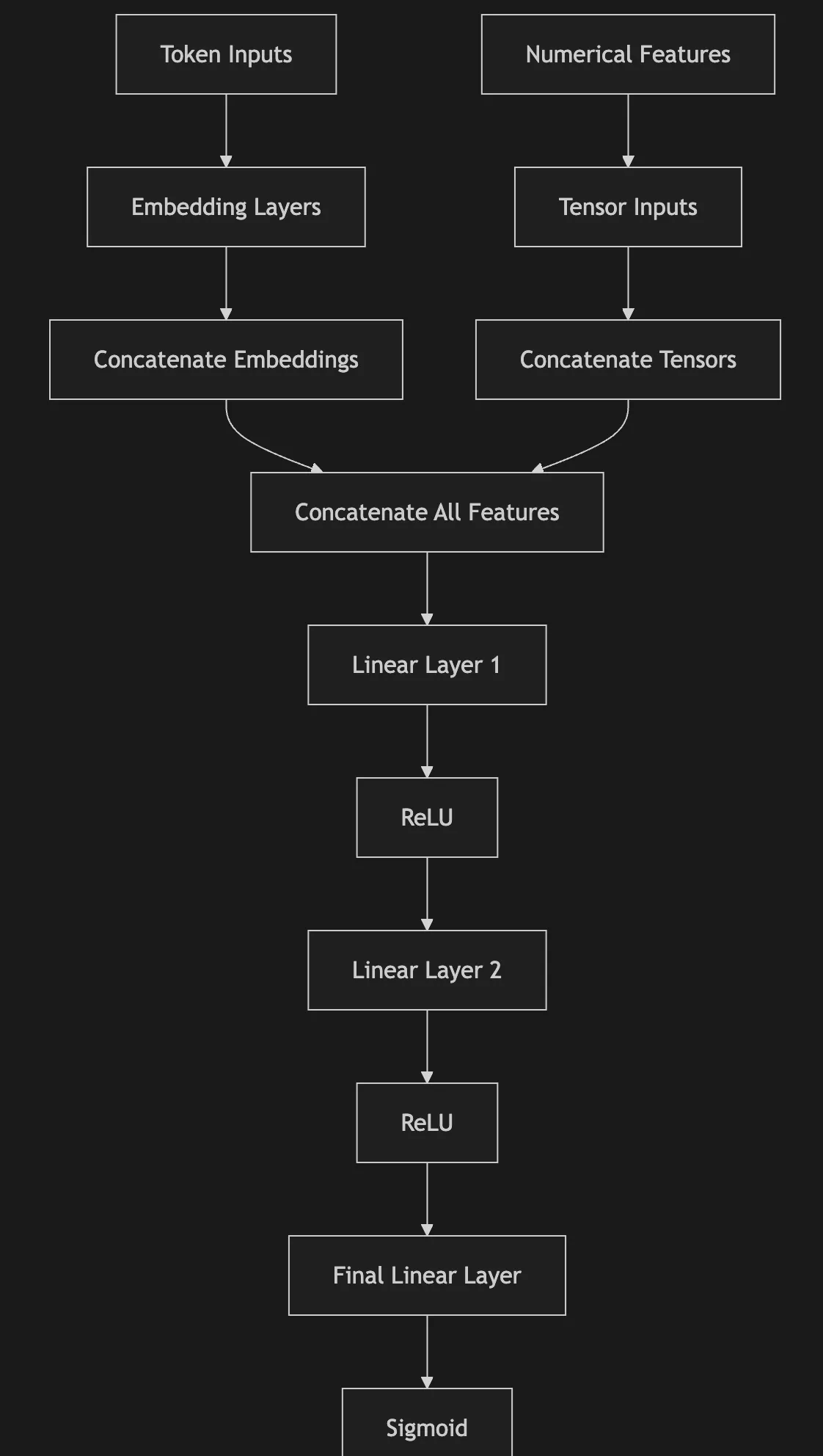
Figure 1. Model Architecture of the Opportunity Scoring Classifier
The model itself is actually really simple. See Figure 1 for the details. Our token values are handled with embedding layers and the outputs of these are then concatenated together with the numerical tensors from the numerical features. We then pass this long vector through 2 fully connected linear layers, separated by rectified linear units and a final linear layer projects the output as a single logit to which a sigmoid function is applied to obtain a probability.
Now you can add batch normalisation, but in practice I’ve found that it can actually be detrimental to performance so my preference is to not use it.
Training Process
Those of you who have read some of my other posts will know that I’m a big fan of 1-cycle scheduling and that would be my go to scheduling profile of choice. I would normally run this type of model with a batch size of 320, with an AdamW optimizer over 50 epochs and measure the loss of the validation set at the end of each training epoch. At the end of the training schedule I’ll select the model that has the lowest validation loss ( across all the training epochs ) and use that as a release candidate that will be tested on the test set to ensure there is consistency between validation and test sets. I use the Binary Cross Entropy Loss as an a loss function.
Regularisation
Unlike a more elaborate architecture like TabNet this architecture is simple, but powerful and I’ve found that using a lot of regularisation really helps to produce consistently good results. There are 3 regularisation techniques that I find work well in combination.
-
Dropout (usually in a range of 0.3 - 0.5)
-
Weight decay ( ~ 0.01 - 0.1 )
-
Embedding dropout (0.3 - 0.5)
Embedding dropout is not very well known so it’s worth me discussing it briefly here. The idea is that with some random probability p each embedding has all its values set to zero. Because each text based feature has its own embedding this is the equivalent of switching off an entire feature. I’ve found that empirically it does seem to improve performance.
Results
One company ran a test which pitched Einstein against a model that we had created based on the design outlined in this post. The test was run over a 3 month period and their feedback was that this approach outperformed Einstein opportunity by 6 percentage points ( 69% vs 75% ).
Our own internal tests showed that this approach is superior to a model based only on the Opportunity (ie no Opportunity History). Improving accuracy on a reasonably balanced dataset from 65% up to 77%.
Conclusion
That concludes our exploration of creating custom neural net models on salesforce opportunity data. Obviously this approach could be used in other use cases such as predict churn or lead quality. The intention was to give you an overview of what I’ve found to work successfully over the past 8 years.
If you’d like to discuss how custom models can help provide you with predictive insights into your business then we’d love to hear from you. Please do get in touch